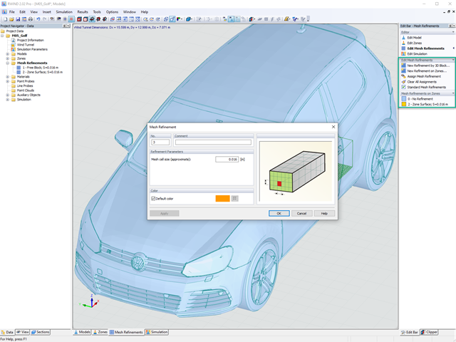
Do you already know the editor for mesh refinement control? It is a great help for your work! Why? It's easy – it gives you the following options:
- Graphic visualization of the areas with mesh refinements
- Mesh refinement of zones
- Deactivating the standard 3D solid mesh refinement with transversion into the corresponding manual 3D mesh refinements.
These options help you to formulate a suitable rule for meshing the entire model, even for the models with unusual dimensions. Use the editor to efficiently define small model details on large buildings or detailed meshing areas in the coating area of the model. You will be amazed!
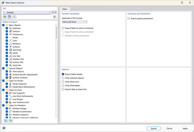
Did you know? You can export all RFEM/RSTAB tables with the results individually or all at once directly into an Excel table or as a CSV file. There are several options available to you:
- With table headers
- Selected objects only
- Filled rows only
- Only filled tables
- Export data as plain text
This way, the program allows you to control and clearly manage the exported data. You can export the stored formulas directly in the table or as a separate table, as in the case of the used parameters.
Have you ever wondered if you can render without a graphics card? We have the answer! Software rendering for alternative image synthesis without the support of a graphics card is possible. You can easily control this solution with the Windows command scripts:
- Enable Software Renderer.cmd (switch on)
- Disable Software Renderer.cmd (switch off)
in the program folder C:\Program Files\Dlubal\RFEM 6.02\bin.
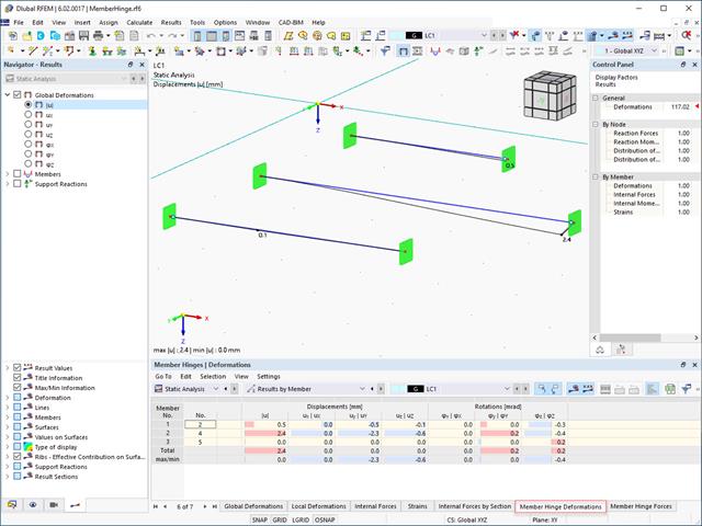
The results for members can be displayed graphically, using the Member Hinges navigator category. The numerical results of member hinges can be found in the Results by Member table category. The Member Hinge Deformations and Member Hinge Forces tables are available for the analysis and documentation of the deformation and force results in the area of member hinges.
The table lists the deformations and forces of each member for the locations specified in the Results Table Manager. There, you can also control which extreme values are displayed.
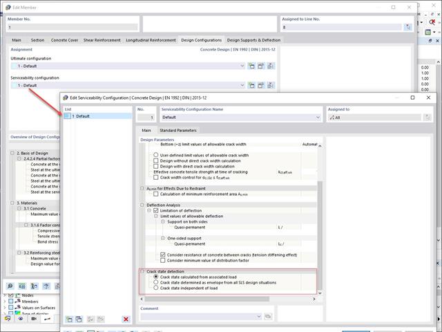
Various design parameters of the cross-sections can be adjusted in the serviceability limit state configuration. The applied cross-section condition for the deformation and crack width analysis can be controlled there.
For this, the following settings can be activated:
- Crack state calculated from associated load
- Crack state determined as an envelope from all SLS design situations
- Cracked state of cross-section - independent of load
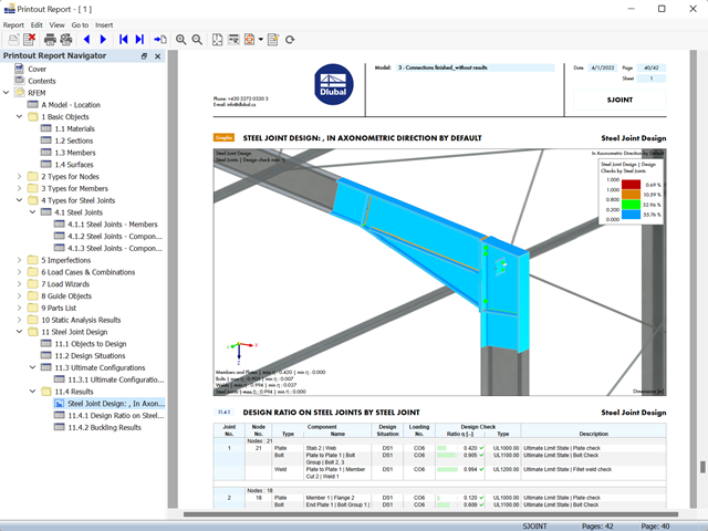
- The results of the connection design can be entered in the printout report
- When creating a new printout report, select the items added from the Steel Joints Add-on
- Use the tool 'Print Graphics to Printout Report' to insert graphics with the results of the connection, including the control panel, into the report
- Printout report contains the specifications of the connection components, design parameters, results and graphics

Did you know? In contrast to other material models, the stress-strain diagram for this material model is not antimetric to the origin. You can use this material model to simulate the behavior of steel fiber-reinforced concrete, for example. Find detailed information about modeling steel fiber-reinforced concrete in the technical article about Determining the material properties of steel-fiber-reinforced concrete.
In this material model, the isotropic stiffness is reduced with a scalar damage parameter. This damage parameter is determined from the stress curve defined in the Diagram. The direction of the principal stresses is not taken into account. Rather, the damage occurs in the direction of the equivalent strain, which also covers the third direction perpendicular to the plane. The tension and compression area of the stress tensor is treated separately. In this case, different damage parameters apply.
The "Reference element size" controls how the strain in the crack area is scaled to the length of the element. With the default value zero, no scaling is performed. Thus, the material behavior of the steel fiber concrete is modeled realistically.
Find more information about the theoretical background of the "Isotropic Damage" material model in the technical article describing the Nonlinear Material Model Damage.
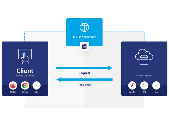
WebService and API provide you various scope of application. We have summarized some ideas as to how WebService and API can support your company:
- Creating additional applications for RFEM 6, RSTAB 9, and RSECTION 1
- Possibility to make the workflows more efficient (for example, model definition and input) and to integrate RFEM 6, RSTAB 9, and RSECTION 1 into your company applications
- Simulating and calculating several design options
- Running optimization algorithms for size, shape, and/or topology
- Accessing the calculation results
- Generation of printout reports in the PDF format
The level of quality of the work is automatically increased not only by the algorithmic model definitions, but also by:
- Extending / consolidating RFEM 6, RSTAB 9, and RSECTION 1 with your own controls
- Increased interoperability between the individual software used to complete a project
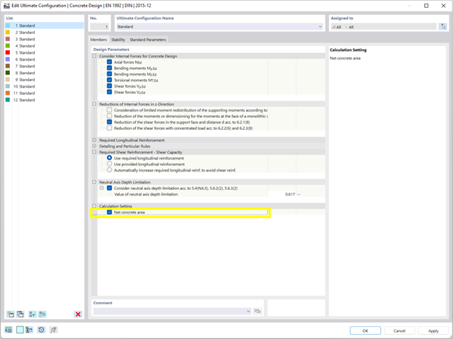
During the cross-section design, you can directly control whether the concrete surface is applied behind the reinforcing bars or is subtracted from the concrete cross-section. You can use the design of the net concrete cross-section especially in the case you deal with a highly reinforced cross-section.

Reinforced concrete usually answers the question "How much can you carry?" simply with "Yes". Nevertheless, you need a three-dimensional moment-moment-axial force interaction diagram for the graphical output of the ultimate limit state of reinforced concrete cross-sections. The Dlubal structural analysis software offers you just that.
With the additional display of the load action, you can easily recognize or visualize whether the limit resistance of a reinforced concrete cross-section is exceeded. Since you can control the diagram properties, you can customize the appearance of the My-Mz-N diagram to suit your needs.
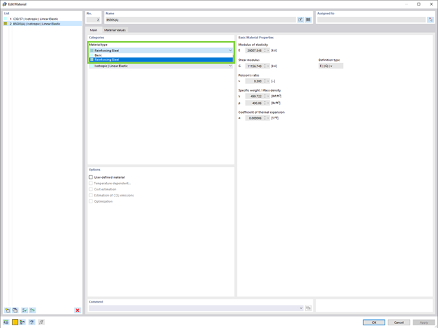
Keep track of your design checks. The material type of a material is used to clearly define the design-relevant properties.
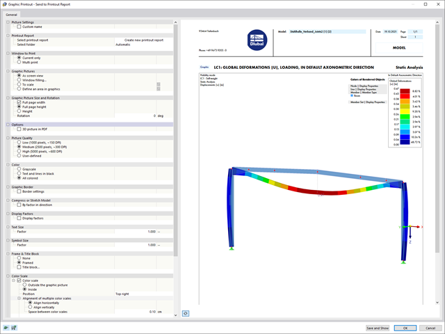
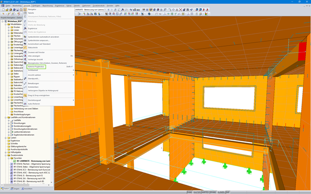
Various new options make it easier for you to print graphics in the future. Your new graphic printout dialog now includes:
- Library-controlled mass print function for all program graphics
- User-defined print area selection
- 3D function for later 3D functionalities in the final PDF
- Automatic separation of images for scale prints and the function for displaying an overview image
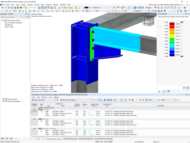
Do you work with steel connections? The Steel Joints add-on for RFEM supports you when analyzing steel connections by using an FE model. In this case, the modeling runs fully automatically in the background. Nevertheless, you can control this process via the simple and familiar input of components. You can then use the loads determined on the FE model for your design of the components according to EN 1993‑1‑8 (including National Annexes).
More About Steel Joints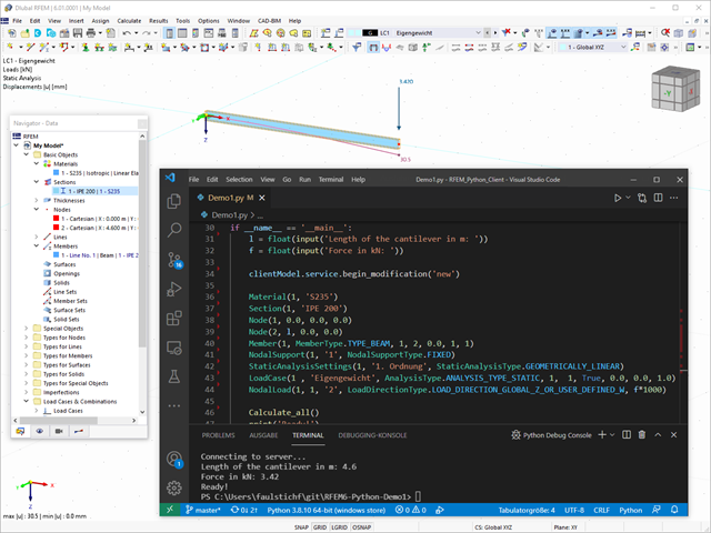
Webservice and API opens up a wide range of new possibilities for you. You can create your own desktop or web-based applications by controlling all objects included in RFEM 6 and RSTAB 9. By providing libraries and functions, you can develop your own design checks, effective modeling of parametric structures, as well as optimization and automation processes using the programming languages Python and C#. Does that sound exciting to you? Then find out more here!
More About Webservice and API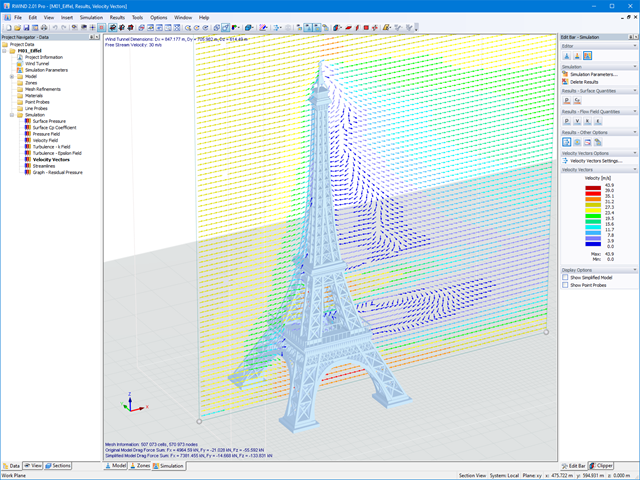
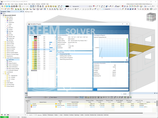
RWIND Basic uses a numerical CFD model (Computational Fluid Dynamics) to simulate wind flows around your objects using a digital wind tunnel. The simulation process determines specific wind loads acting on your model surfaces from the flow result around the model.
A 3D volume mesh is responsible for the simulation itself. For this, RWIND Basic performs an automatic meshing on the basis of freely definable control parameters. For the calculation of wind flows, RWIND Basic provides you with a stationary solve and RWIND Pro provides a transient solver for incompressible turbulent flows. Surface pressures resulting from the flow results are extrapolated onto the model for each time step.
Technology takes you further, also in your daily work with RFEM / RSTAB. The new API technology Webservice allows you to create your own desktop or web-based applications by controlling all objects included in RFEM 6 / RSTAB 9. Entire libraries and numerous functions are available to you. Thus, you can easily perform your own design checks, effective modeling of parametric structures, and optimization and automation processes using the programming languages Python and C#. Dlubal Software makes your work easier and more convenient. Check it out now!
WebService and API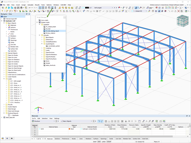
Navigate easily and intuitively. Use the script manager to control all input elements using JavaScript via the console or saved scripts.
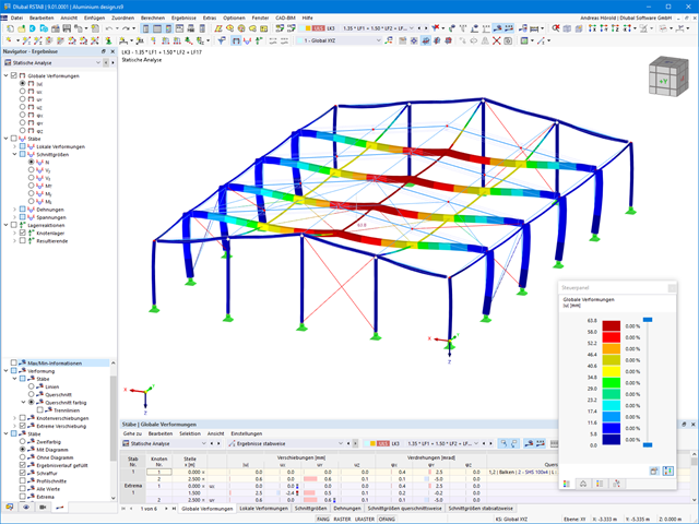
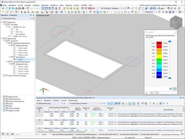
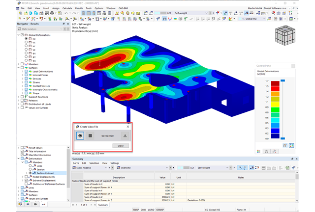
Also, on the rendered model, you see your results in a clear color display. This allows you to precisely recognize the deformation or internal forces of a member, for example. If you want to set the colors and value ranges, you can do so in the control panel.
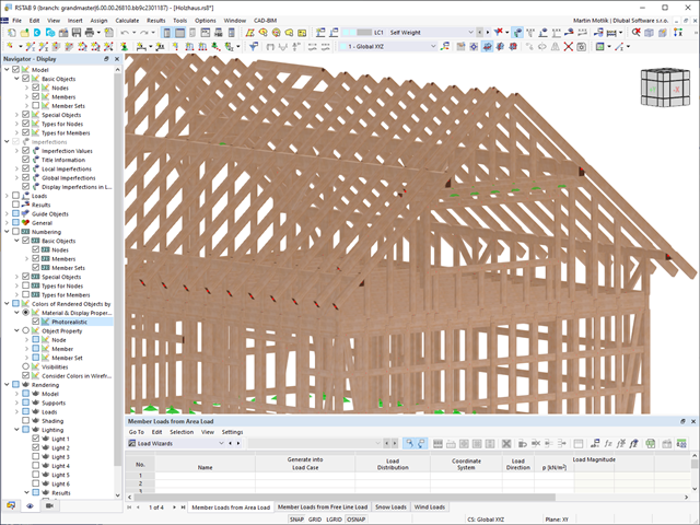
The model is rendered photorealistically (optionally with textures). This gives you the advantage that you always have immediate control of the input. You can freely adjust the display colors and save them separately for the screen as well as for the printout.
Go to Explanatory Video
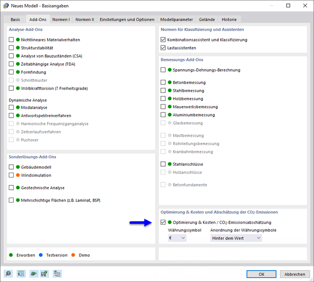
Did you know that The structural optimization in the programs RFEM and RSTAB is a completion of the parametric input. It is a parallel process beside the actual model calculation with all its regular calculation and design definitions. The add-on assumes that your model or block is built with a parametric context and is controlled in its entirety by global control parameters of the "optimization" type. Therefore, these control parameters have a lower and upper limit and a step size to delimit the optimization range. If you want to find optimal values for the control parameters, you have to specify an optimization criterion (for example, minimum weight) with the selection of an optimization method (for example, particle swarm optimization).
You can already find the cost and CO2 emission estimation in the material definitions. You can activate both options individually in each material definition. The estimation is based on a unit for unit cost or unit emission for members, surfaces, and solids. In this case, you can select whether to specify the units by weight, volume, or area.
Both optimization methods have one thing in common. At the end of the process, they provide you with a list of model mutations from the stored data. Here you can find the details of the controlling optimization result and the associated value assignment of the optimization parameters. This list is organized in descending order. You can find the assumed best solution shown in the first line. For this, the optimization result with its determined value assignment is closest to the optimization criterion. All add-on results have a utilization < 1. Furthermore, once the analysis is completed, the program will adjust the value assignment to that of the optimal solution for the optimization parameters in the global parameter list.
In the material dialog boxes, you can find the additional tabs "Cost Estimation" and "Estimation of CO2 Emissions". They show you the individual estimated sums of the assigned members, surfaces, and solids per unit weight, volume, and area. Furthermore, these tabs show the total cost and emission of all assigned materials. This gives you a good overview of your project.
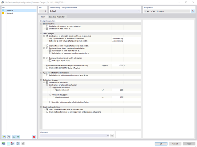
Are you looking for a deformation calculation? Check the Serviceability Configuration, where it can be activated. You can also control the consideration of long-term effects (creep and shrinkage) and tension stiffening between cracks in the dialog box above. The creep coefficient and shrinkage strain are calculated using the specified input parameters, or you can define them individually.
Furthermore, you can specify the deformation limit value individually for each structural component. The max. deformation is defined as the allowable limit value. In addition, you have to specify whether you want to use the undeformed or the deformed system for the design check.
- Import of relevant information and results from RFEM
- Integrated, editable material and section library
- Sensible and complete presetting of input parameters
- Punching design on columns (all section shapes), wall ends, and wall corners
- Automatic recognition of the punching node position from an RFEM model
- Detection of curves or splines as a boundary of the control perimeter
- Automatic consideration of all slab openings defined in the RFEM model
- Construction and graphical display of the control perimeter
- Optional design with unsmoothed shear stress along the control perimeter that corresponds to the actual shear stress distribution in the FE model
- Determination of the load increment factor β via full-plastic shear distribution as constant factors according to EN 1992‑1‑1, Sect. 6.4.3 (3), based on EN 1992‑1‑1, Fig. 6.21N, or by a user‑defined specification
- Numerical and graphical display of results (3D, 2D, and in sections)
- Punching design of the slab without punching reinforcement
- Qualitative determination of the required punching reinforcement
- Design and analysis of the longitudinal reinforcement
- Complete integration of results in an RFEM printout report
You have two options in RFEM. On the one hand, you can determine the punching load from a single load (from column/loading/nodal support) and the smoothed or unsmoothed shear force distribution along the control perimeter. On the other hand, you can specify them as user-defined.
Calculate the design ratio of the punching shear resistance without punching reinforcement as a design criterion and the program will deliver you the corresponding result. In the case of exceeding the punching shear resistance without punching reinforcement, the program determines the required punching reinforcement as well as the required longitudinal reinforcement for you.
Also on the rendered model, you see your results in a clear color display. Thus, you can exactly recognize the rotation of a member or the stress distribution in a surface, for example. If you want to set the colors and value ranges, you can easily do so in the control panel.
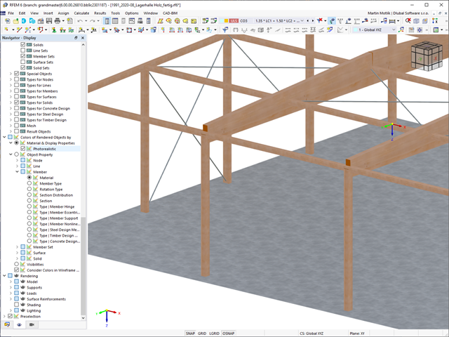
Always keep an eye on your model. Due to the photorealistic rendering (optionally with textures), you always have immediate control of your input. You can freely adjust the display colors and save them separately for screen and printout.
Go to Explanatory Video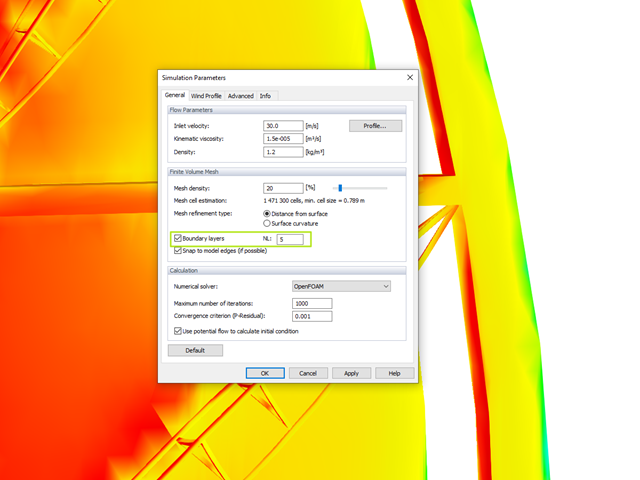
The meshing algorithm of RWIND Simulation uses the boundary layer option to mesh the area near the model surface with a voluminous layer mesh. The number of layers is controlled by a user-defined parameter.
This fine mesh in the area of the model surface helps to represent the wind velocity close to the surface.
With the Camera Fly Mode view option, you can fly through your RFEM and RSTAB structure. Control the direction and speed of the flight with your keyboard. Additionally, you can save the flight through your structure as a video.
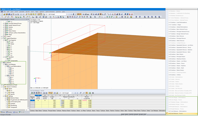
RFEM offers the following tables to display forces and deformations of hinges and releases:
- 4.45 Line Hinges - Deformations
- 4.46 Line Hinges - Forces
- 4.47 Member Hinges - Deformations
- 4.48 Member Hinges - Forces
- 4.49 Nodal Releases - Deformations
- 4.50 Nodal Releases - Forces
- 4.51 Line Releases - Deformations
- 4.52 Line Releases - Forces
The tables can be displayed in the prinout report. Moreover, the results in line hinges and line releases can be displayed graphically. It can be controlled by Project Navigator - Results.
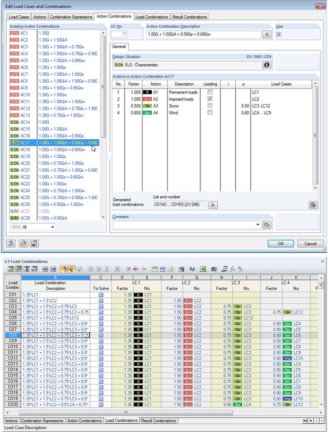
Utilize all the options of the 'Edit Load Cases and Combinations' dialog box to facilitate your work. Here you can automatically create load and result combinations after selecting the corresponding combination expressions. In this clearly arranged dialog box, you can also e.g. to copy, add, or renumber load cases.
Additionally, control the load cases and combinations in Tables 2.1 – 2.6.